Introduction to ss3sim

2024-04-17

This vignette is a good starting place for learning about {ss3sim}.

Overview

{ss3sim} is an R package to simplify the steps needed to generate beautiful simulation output from Stock Synthesis (SS3). If you need help learning R prior to using {ss3sim}, we recommend navigating to the RStudio Blog.

{ss3sim} consists of

• a series of low-level functions that facilitate manipulating Stock Synthesis configuration files, running Stock Synthesis models, and combining the output;
• a few high-level wrapper functions that control simulation experiments, e.g., run_ss3sim(); and
• documentation for the user, e.g., ?change_f, vignettes, issue tracker, and a Discussion board for users and developers to interact.

The developers of {ss3sim} strive to facilitate an inviting place where all individuals feel welcome. Please see the Code of Conduct that we abide by to ensure contributors are valued and Contributor Guidelines for how to contribute.

Stock Synthesis

It seems imperative to first describe Stock Synthesis because without Stock Synthesis there would not be {ss3sim}. Stock Synthesis is an integrated statistical catch-at-age model written in ADMB. The software is widely used across the globe and has been around for 40+ years.

The inspiration for {ss3sim} came from Hui-Hua Lee’s hooilator software. hooliator parsed data.ss_new files into multiple files and created a consistent directory structure to store the results. As of Stock Synthesis 3.30.19, the need to separate out the data.ss_new file into separate files is no longer necessary because Stock Synthesis itself now ports the output into separate files, i.e., the echoed data are in data_echo.ss_new, the expected values are in data_expval.ss, and simulated data sets are in data_boot_**N.ss. See the section on output files in the Stock Synthesis manual for more detailed information. {ss3sim} finishes the creation of simulation-specific directories similar to the directory structure that was created by hooliator. {ss3sim} adds functionality to sample from the expected values such that simulations need not rely on bootstrapped values provided in data_boot_**N.ss. With a plethora of simulation output stored in structured folders, there was an imminent need for functions to visualize the results. {ggplot2} was gaining traction at the time and shaped how we thought about things, including our mission statement and example output.

{ss3sim} is just a minor part of the suite of functionality available for Stock Synthesis. See the Stock Synthesis website for a list of additional software.

Installation

Installing {ss3sim}

{ss3sim} is available on CRAN and GitHub and can be run on OS X, Windows, or Linux. The GitHub branch “main” contains the newest features, which are more than likely not available on CRAN. We recommend using the GitHub version because development of {ss3sim} is very fluid and new features are added almost monthly, whereas CRAN submissions tend to be bi-annual.

Run the following code to install {ss3sim} and load it into your workspace. You will not need to install {ss3sim} every time but it is a good idea to ensure it is up to date. If you are installing from GitHub, you may need to install {remotes} or {pak}, utils::install.packges("pak"), before installing {ss3sim} if you do not already have {devtools} installed. If your current version of {ss3sim} is up to date, R will let you know and prompt you if you want to override the current installation.

pak::pkg_install(
  pkg = "ss3sim/ss3sim",
  # pkg = "ss3sim" # CRAN version
  dependencies = TRUE
)

# Load the package
library("ss3sim")

The following code demonstrates how to access the {ss3sim} documentation within R. You can also view the vignettes online.

?ss3sim
utils::help(package = "ss3sim")
utils::browseVignettes("ss3sim")

Installing Stock Synthesis

{ss3sim} relies the Stock Synthesis executable being available to the operating system. Thus, the executable must be in your path, which is a list of directories that your operating system has access to and searches through when a program is called. Having Stock Synthesis in your path allows {ss3sim} to use the name of the single, saved executable instead of requiring the full path or copying the executable to every local directory before calling it, which saves on space because the Stock Synthesis binary is about 6 MB. This functionality of not copying the executable works even when running Stock Synthesis in parallel.

{ss3sim} will first look to see if the executable is available in your R library using system.file("bin", package = "ss3sim"). The previous will only lead to a viable file path if you are using the GitHub version of {ss3sim} because the distribution of executables is not allowed on CRAN. If the location is not returned from system.file, R will look for the executable in your path. This hierarchy is important for understanding which version of Stock Synthesis is being used because you might already have a version of Stock Synthesis in your path.

{ss3sim} was originally based on Stock Synthesis 3.24O (Anderson et al. 2014) and did not immediately update to use Stock Synthesis 3.30. In 2019, {ss3sim} was updated to use Stock Synthesis 3.30, and users can count on future versions of {ss3sim} being up to date with the newest version of Stock Synthesis. Stock Synthesis will end development with major-version three but minor versions will continue to be updated for quite some time.

If you are using the CRAN version of {ss3sim}, reference Getting Started with Stock Synthesis for instructions on how to put Stock Synthesis in your path. Or, you can mimic the directory structure of the GitHub version of {ss3sim} and place the executable in the appropriate folder below

├──library
|  └──ss3sim
|  |  ├──bin
|  |  |  ├──Linux64
|  |  |  ├──MacOS
|  |  |  └──Windows64

But, the executable will need to be updated every time you reinstall {ss3sim}.

Compiled Stock Synthesis executables are available for multiple operating systems on GitHub or in GitHub actions in the Stock Synthesis repository.

Installing dependent R packages

Installing {ss3sim} will install all of the necessary dependent packages without users needing to do anything extra. But, for completeness and as an acknowledgement, below we highlight a few packages that are essential for running {ss3sim}.

{r4ss}

If you are using the GitHub version of {ss3sim}, R will install the GitHub version of {r4ss}. If you are using the CRAN version of {ss3sim}, R will install the CRAN version of {r4ss}. Both methods will check to make sure that you have the appropriate version of {r4ss} in your R library given the mirror you are using. Feel free to install {r4ss} directly via

pak::pkg_install("r4ss/r4ss", dependencies = TRUE)

But, make sure you do it before loading {ss3sim}. If you forget, you can use devtools::unload(package = "ss3sim") and then reinstall {r4ss}.

{ggplot2}

{ggplot2} uses the Grammar of Graphics to decoratively create images that represent things in a tidy way. We do not force users to use {ggplot2}. All output is available in *.csv files and can be visualized using base R if you prefer. The easiest way to get {ggplot2} is to install the whole tidyverse suite.

pak::pkg_install("tidyverse")

Scenarios

Simulations are composed of scenarios, i.e., unique sets of changes to the OM and EM. run_ss3sim() uses simdf to specify the setup of scenarios within a simulation. simdf stands for simulation data frame. The rows of the data frame store scenario-level information. The columns of the data frame store function arguments. Arguments can be direct arguments of ss3sim_base() or functions called by ss3sim_base() such as change_f(). You only need to specify columns for the arguments that you want to change. That is, you do not have to have a column for every argument of all functions called by ss3sim_base(). To get a feel for the columns needed in the simdf data frame run the following code, where the output can be saved and used to build simdf.

simdf <- setup_scenarios_defaults()

Column entries of simdf need to be quoted if they are to be evaluated later, e.g., "seq(1,10,by=2)" and "c('NatM_uniform_Fem_GP_1', 'L_at_Amin_Fem_GP_1')". Scalar values can numeric. Use single quotes inside of double quotes to quote text. Developers of {ss3sim} are working on a better, more tidyverse-like non-standard evaluation method such that quotes will not be needed. Feel free to reach out if you would like to help with this effort or have ideas on how to make it work better.

Column names of simdf are key. You can specify any input argument to ss3sim_base() as a column of simdf.

{ss3sim} function	Argument	Description
ss3sim_base	bias_adjust	Perform bias adjustment

For functions that are called by ss3sim_base() you need to use the following rules to create appropriate column names:

• abbreviation of the function name (see the table below),
• full stop,
• the argument name,
• full stop, and
• integers to specify which fleet the column pertains to.

For example, cf.years.1 passes information to the year argument of change_f() for fleet 1. cf.years.2 passes information to the year argument of change_f() for fleet 2. Function abbreviations are as follows:

{ss3sim} function	Prefix	Description
change_f()	cf.	Fishing mortality
change_e()	ce.	Estimation
change_o()	co.	Operating model
change_tv()	ct.	Time-varying OM parameter
change_data()	cd.	Available OM data, bins, etc.
change_em_binning()	cb.	Available EM data bins
change_retro()	cr.	Retrospective year
sample_index()	si.	Index data
sample_agecomp()	sa.	Age-composition data
sample_lcomp()	sl.	Length-composition data
sample_calcomp()	sc.	Conditional age-at-length data
sample_mlacomp()	sm.	Mean length-at-age data
sample_wtatage()	sw.	Weight-at-age data

Currently, fishing mortality, indices of abundance, and either age- or length-composition data are mandatory for a scenario.

File structure

Input file structure

{ss3sim} comes with a generic, built-in operating model (OM) and estimation method (EM). The life history for these available files is based on a cod-like fish. You can peruse the files if you have {ss3sim} installed here

system.file("extdata/models", package = "ss3sim")

These model files can be used as is, modified, or replaced. For more details on how to modify or replace the default models, see the vignettes on modifying model setups and creating your own OM and EMs.

You can have as many OMs and EMs as you want in your simulation. The collection of files for each OM and EM should be in its own directory, just like the example OM and EM.

Simulation file structure

Internally, copy_ss3models() creates the directory structure for the simulations. After you run a simulation, directories will be created in your working directory. Inside your working directory, the structure will look like

  scenarioA/1/om
  scenarioA/1/em
  scenarioA/2/om
  scenarioA/2/em
  scenarioB/1/om
  scenarioB/1/em
  ...

The integer values after the scenario represent iterations; the total number of iterations is specified by the user. The OM and EM directories are copied into individual directories for an iteration. Note that the supplied OM and EM directories will be renamed om and em within each iteration. There will be some additional directories if you are using bias adjustment. See ss3sim_base() for more information on bias adjustment. You can name the scenarios any combination of character values or use the default naming system within {ss3sim} that uses the date and time.

The supplied OM and EM directories are checked to ensure

• they contain the minimal files,
• the filenames are lowercase,
• the data file is named ss.dat,
• the control files are named om.ctl or em.ctl, and
• the starter files are adjusted to reflect these file names.

Example simulations with {ss3sim}

The example is based on the cod-like species in the papers Ono et al. (2015) and Johnson et al. (2015), both of which used {ss3sim}. All of the required files for this example are contained within {ss3sim}. This example is a 2x2 design, testing

1. the effect of high and low precision on the index of abundance provided by the survey and
2. the effect of fixing versus estimating natural mortality (\(M\)).

Setting up the example

First we will create df, a data frame for run_ss3sim(simdf = df).

# Use the boiler-plate data frame available in {ss3sim} for 2 scenarios
df <- setup_scenarios_defaults(nscenarios = 2)
# Turn off bias adjustment and use default settings in cod EM model
df[, "bias_adjust"] <- FALSE

Fishing mortality

Fishing mortality, \(F\), is set to a constant percentage of \(F\) at maximum sustainable yield, \(F_\mathrm{MSY}\), from when the fishery starts in year 26 until the end of the simulation in year 100.

# Display the default fishing mortality settings
df[, grep("^cf\\.", colnames(df))]
#>   cf.years.1      cf.fvals.1
#> 1     26:100 rep(0.1052, 75)
#> 2     26:100 rep(0.1052, 75)

Composition data

Refer to the help files ?sample_lcomp and ?sample_agecomp for detailed information on these functions. The sampling theory is described in the age- and length-composition sampling section.

The default simdf contains sampling protocols for composition data.

# Display the default composition-data settings
# sa is for ages and sl is for lengths
df[, grep("^s[al]\\.", colnames(df))]
#>   sl.Nsamp.1 sl.years.1 sl.Nsamp.2           sl.years.2 sl.cpar sa.Nsamp.1
#> 1         50     26:100        100 seq(62, 100, by = 2)    NULL         50
#> 2         50     26:100        100 seq(62, 100, by = 2)    NULL         50
#>   sa.years.1 sa.Nsamp.2           sa.years.2 sa.cpar
#> 1     26:100        100 seq(62, 100, by = 2)    NULL
#> 2     26:100        100 seq(62, 100, by = 2)    NULL

Survey index of abundance

To investigate the effect of different levels of precision on the survey index of abundance, we will manipulate sds_obs of sample_index(). This argument ultimately refers to the standard error of the natural log of yearly index values, as defined in Stock Synthesis. In the first scenario sds_obs = 0.1. In the second scenario sds_obs = 0.4.

# Create a biennial survey starting in year 76 and ending in the terminal year
df[, "si.years.2"] <- "seq(76, 100, by = 2)"
# Set sd of observation error for each scenario
df[, "si.sds_obs.2"] <- c(0.1, 0.4)

Estimating parameters

To investigate the effect of fixing versus estimating \(M\), df must be augmented to call change_e(). Using par_phase one can turn a parameter on and off in the EM, where negative phases tells Stock Synthesis to not estimate the parameter. The second scenario will estimate \(M\) in phase 3.

df <- rbind(df, df)
df[, "ce.par_name"] <- "NatM_uniform_Fem_GP_1"
df[, "ce.par_int"] <- NA
# Set the phase for estimating natural mortality
df[, "ce.par_phase"] <- rep(c(-1, 3), each = 2)
# Name the scenarios
df[, "scenarios"] <- c(
  "D0-E0-F0-cod", "D1-E0-F0-cod",
  "D0-E1-F0-cod", "D1-E1-F0-cod"
)

Visualizing the results

Five iterations is unrealistic for a manuscript but saves time and disk space here. You can assess how many iterations are needed to stabilize the results using plot_cummean(), which plots the mean relative error on the y as additional iterations. The goal is to run plenty of iterations, such that additional iterations no longer appreciably flatten the curve towards a relative error of zero.

iterations <- 1:5
scname <- run_ss3sim(iterations = iterations, simdf = df)

A quick test that can be helpful is visualizing the patterns of spawning stock biomass from the OM and the EM using r4ss.

r_om <- r4ss::SS_output(file.path(scname[1], "1", "om"),
  verbose = FALSE, printstats = FALSE, covar = FALSE
)
r_em <- r4ss::SS_output(file.path(scname[1], "1", "em"),
  verbose = FALSE, printstats = FALSE, covar = FALSE
)
r4ss::SSplotComparisons(r4ss::SSsummarize(list(r_om, r_em)),
  legendlabels = c("OM", "EM"), subplots = 1
)

Each iteration is unique because of process error included through normally-distributed recruitment deviations. Thus, if you were to plot the OMs from iteration one and two using r4ss::SSplotComparisons() there would be clear annual differences. Deviations are generated for each iteration in your simulation and used across scenarios. Using the same deviations for iteration one of each scenario, and a different set of deviations for each additional iteration, facilitates comparisons across scenarios. The default distribution in {ss3sim} has a mean of -0.5 and a standard deviation of 1 (bias-corrected standard-normal deviations). These deviations are then scaled by the level of recruitment variability specified in the OM with \(\sigma_r\). If you would like to specify your own deviations, you can pass them using user_recdevs. See the next section on self tests for an example of user_recdevs.

Self test to check for bias

Self testing is a crucial step of any simulation study to confirm that parameters are identifiable. One way to ensure the dynamics are what they were intended to be is to set up an EM that is similar to the OM and include minimal process and observation error in the OM. We recommend minimal and not zero error. Stability issues will arise in non-linear, integrated models that assume error structures when there is in fact none.

Setup self test

We will start by setting up a 200 row (number of years) by 20 column (number of iterations) matrix of recruitment deviations, where all values are set to zero.

Then, we will set up OM and EM files with the standard deviation of recruitment variability, SR_sigmaR \(\sigma_R\), set to 0.001. To do this, the data frame that controls the scenarios must specify par_name = SR_sigmaR (the Stock Synthesis parameter name) and par_int = 0.001 (the initial value) for both change_o and change_e for the OM and EM, respectively. To minimize observation error on the survey index, we will create a standard deviation on the survey observation error of 0.001. Finally, we will fix \(M\) at the true value and estimate it in phase 3 as we did before.

df <- setup_scenarios_defaults(nscenarios = 2)
df[, "user_recdevs"] <- "matrix(0, nrow = 200, ncol = 20)"
df[, "co.par_name"] <- "SR_sigmaR"
df[, "co.par_int"] <- 0.001
df[1, "ce.par_name"] <- "SR_sigmaR"
df[1, "ce.par_int"] <- 0.001
df[1, "ce.par_phase"] <- -1
df[, "ce.forecast_num"] <- 0
df[, "si.years.2"] <- "seq(60, 100, by = 2)"
df[, "si.sds_obs.2"] <- 0.001
df[2, "ce.par_name"] <- 'c("SR_sigmaR", "NatM_uniform_Fem_GP_1")'
df[2, "ce.par_int"] <- "c(0.001, NA)"
df[2, "ce.par_phase"] <- "c(-1, 3)"
df[, "scenarios"] <- c("D1-E100-F0-cod", "D1-E101-F0-M1-cod")
df[, "bias_adjust"] <- FALSE

Run self-test

iterations <- 1:5
scname_det <- run_ss3sim(iterations = iterations, simdf = df)

Checking output

Check the model results to make sure that the EM returns the same parameters as the OM. get_results_all() should be sufficient here, which will produce csv files that you can use to check parameter estimates. For more details see the section on model output.

Beautiful output

.csv files

get_results_all() reads in a set of scenarios and combines the output into .csv files, e.g., ss3sim_scalar.csv and ss3sim_ts.csv. The scalar file contains values for which there is a single estimated value, e.g., MSY. The ts file refers to values for which there are time series of estimated values, e.g., biomass for each year.

Parameter names in these files will not always be the same across simulations because names are dependent on OM and EM settings. For example, an EM with age-specific natural mortality will have multiple natural mortality parameters each with a different name based on the age they pertain to. get_results_all() accommodates this by using the parameter name assigned by Stock Synthesis rather than attempting to standardize names.

Originally, {ss3sim} provided the results using a wide-table format, with individual columns for each OM and EM parameter along with some summary information for each scenario. In May of 2020 we changed to providing results using a tidier long format.

get_results_all(
  overwrite_files = TRUE,
  user_scenarios = c(scname, scname_det)
)
# Read in the data frames stored in the csv files
scalar_dat <- read.csv("ss3sim_scalar.csv")
ts_dat <- read.csv("ss3sim_ts.csv")

If you would like to follow along with the rest of the vignette without running the simulations detailed above, you can load a saved version of the output.

data("scalar_dat", package = "ss3sim")
data("ts_dat", package = "ss3sim")

Post-processing of results

Calculate the relative error (RE)

scalar_dat <- calculate_re(scalar_dat)
#> Warning in (function (..., deparse.level = 1) : number of columns of result is
#> not a multiple of vector length (arg 1)
ts_dat <- calculate_re(ts_dat)
#> Warning in (function (..., deparse.level = 1) : number of columns of result is
#> not a multiple of vector length (arg 1)

Merge scalar and time series

The gradient information is in the scalar file. Merging the scalar and the time series can help add details to figures.

scalar_dat[, "D"] <- gsub(
  pattern = "D([0-9]+)-.+",
  replacement = "D\\1",
  scalar_dat[, "scenario"]
)
scalar_dat[, "E"] <- ifelse(
  test = scalar_dat$NatM_uniform_Fem_GP_1_em == 0.2,
  "fix M",
  "estimate M"
)
ts_dat <- merge(
  x = dplyr::select(ts_dat, -E),
  y = scalar_dat[, c("scenario", "iteration", "max_grad", "D", "E")]
)

Separate the deterministic from the stochastic runs

ts_dat_sto <- ts_dat[grepl("E[0-1]-", ts_dat[, "scenario"]), ]
scalar_dat_long <- scalar_dat
colnames(scalar_dat_long) <- gsub(
  pattern = "(.+)_re",
  replacement = "RE _\\1",
  x = colnames(scalar_dat_long)
)
scalar_dat_long <- reshape(scalar_dat_long,
  sep = " _",
  direction = "long",
  varying = grep(" _", colnames(scalar_dat_long)),
  idvar = c("scenario", "iteration"),
  timevar = "parameter"
)

Boxplots

Use the long data to create a multi-panel plot with {ggplot2}.

p <- plot_boxplot(
  scalar_dat_long[
    scalar_dat_long$parameter %in% c("depletion", "SSB_MSY") &
      grepl("E10[0-1]", scalar_dat_long[, "scenario"]),
  ],
  x = "E", y = "RE", re = FALSE,
  horiz = "parameter", print = FALSE
)
print(p)

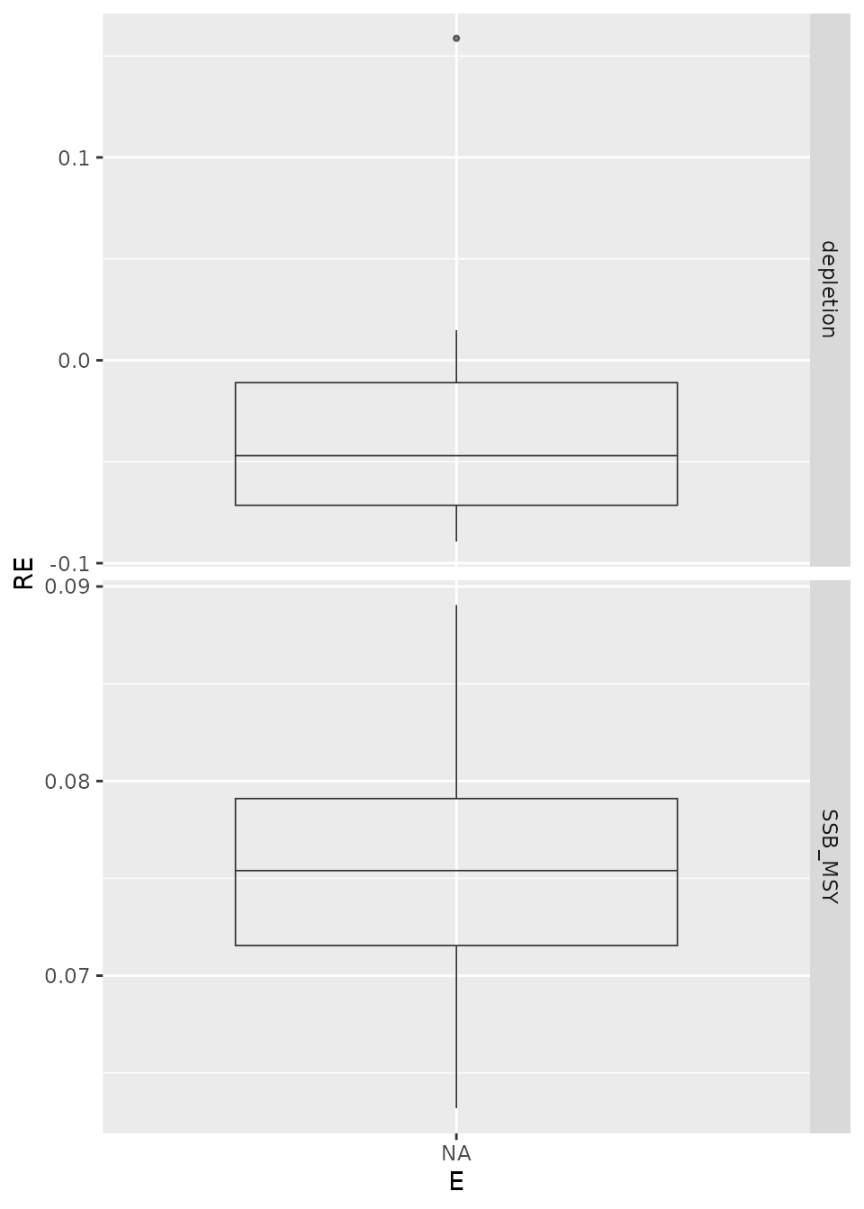
Box plots of the relative error (RE) for deterministic runs. \(M\) is fixed at the true value from the OM (E100) or estimated (E101).

# see plot_points() for another plotting function

While plotting the relative error in estimates of spawning biomass, one can add color to the time series according to the maximum gradient. Small values of the maximum gradient (approximately 0.001 or less) indicate that model convergence is likely. Larger values (greater than 1) indicate that model convergence is unlikely. Results of individual iterations are jittered around the vertical axis to aid in visualization. The following three blocks of code produce Figures~\(\ref{fig:plot-sto-ts}\), \(\ref{fig:ssb-ts-plots}\), and \(\ref{fig:relative-error-boxplots-sto}\).

p <- plot_lines(ts_dat_sto,
  y = "SpawnBio_re",
  vert = "E", horiz = "D", print = FALSE, col = "max_grad"
)
print(p)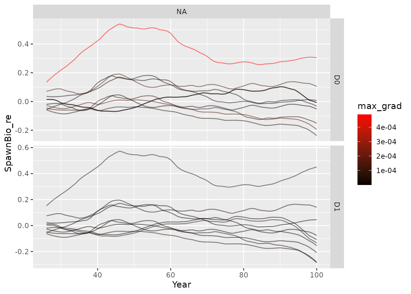

Time series of relative error in spawning stock biomass.

p <- plot_boxplot(
  scalar_dat_long[
    scalar_dat_long$parameter %in% c("depletion", "SSB_MSY") &
      grepl("E[0-1]-", scalar_dat_long$scenario),
  ],
  x = "D", y = "RE", re = FALSE,
  vert = "E", horiz = "parameter", print = FALSE
)
print(p)

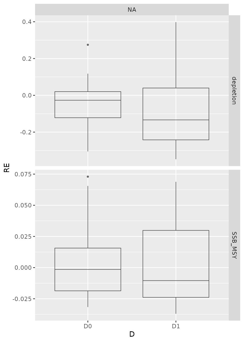
Box plots of relative error (RE) for stochastic runs. \(M\) is fixed at the true value from the OM (E0) or estimated (E1). The standard deviation on the survey index observation error is 0.4 (D1) or 0.1 (D0), representing an increase in survey sampling effort.

Stochasticity

Generating observation error

The sample_*() functions work together to add observation error to the expected values before creating the input .dat file for the EM. Input arguments for these functions have two primary tasks. First, they help decide what types of data are included in the expected values. Second, they dictate how observation error is added to the expectations.

calculate_data_units()

calculate_data_units() is used to modify the OM to include just the data types and quantities that are needed based on the arguments passed to sample_*(). For example, you might wish to fit an EM to conditional length-at-age data with a certain bin structure for certain years and fleets. To do that, expected lengths and ages must be available for appropriate years and fleets at a sufficiently fine bin size. If you have many different scenarios in your simulation, then there will be lots of combinations of expected values that are needed.

Instead of generating every possible combination of years, fleets, etc., which is slow and inefficient, {ss3sim} uses calculate_data_units() to determine the minimal-viable amount of data types needed. For example, if arguments are passed to sample_mlacomp(), then expected values for age and length-at-age are created, even if sample_agecomp() is not being called directly. Similarly, sample_wtatage() leads to expected values for empirical weight-at-age, age-composition, and mean length-at-age data. sample_calcomp() leads to expected values for length- and age-composition data.

Currently, {ss3sim} supports the sampling of the following types of data:

• catch-per-unit effort data with sample_index(),
• length and age compositions with sample_lcomp() and sample_agecomp(),
• mean length (size) at age sample_mlacomp(),
• empirical weight at age with sample_wtatage(), and
• conditional age at length with sample_calcomp().

Distributional assumptions for observation error

In simulations, the true underlying dynamics of the population are known, and therefore, a variety of sampling techniques are possible. Ideal sampling, in the statistical sense, can be done easily. However, there is some question about the realism behind providing the model with this kind of data because it is unlikely to happen in practice (Pennington et al. 2002). One way to generate more realistic data is to use flexible distributions, which allow the user to control the statistical properties, e.g., overdispersion of the data. Another option is to use unmodeled process error, typically in selectivity.

Under perfect mixing of fish and truly random sampling of the population, the age samples would be multinomial. However, in practice fish are never perfectly mixed because fish tend to aggregate by size and age (e.g., Pennington et al. 2002). And, it is difficult to take random samples. Both of these sampling properties can cause the data to have more variance than expected, i.e., be overdispersed, and the effective sample size is smaller than expected (Maunder 2011, Hulson et al. 2012). For example, if a multinomial likelihood is assumed for overdispersed data, the model puts too much weight on those data by thinking they should be less variable than they are, at the cost of fitting other data less well (Maunder 2011). Analysts thus often “tune” their model to find a sample size, i.e., “effective sample size”, that is more appropriate than the “input sample size”. The effective sample size will in theory more accurately reflect the information in the composition data (Francis and Hilborn 2011). In our case, we exactly control how the data are generated and specified in the EM, providing a large amount of flexibility to the user. What is optimal will depend on the questions addressed by a simulation and how the results are meant to be interpreted. We caution users to carefully consider how data are generated and fit.

Indices of abundance

sample_index() facilitates generating relative indices of abundance (catch-per-unit-effort (CPUE) data for fishery fleets). It samples from the biomass trends available for the different fleets to simulate the collection of CPUE and survey index data. The user can specify which fleets are sampled in which years and with what amount of noise. Different fleets will “see” different biomass trends due to differences in selectivity. Catchability for the OM is equal to one, \(q=1\), and thus, the indices are actually absolute indices of (spawning) biomass.

In practice, sampling from the abundance indices is relatively straightforward. The OM .dat file contains the annual biomass values for each fleet, and the sample_index function uses these true values as the mean of a distribution. The function uses a bias-corrected log-normal distribution with expected values given by the OM biomass and a user-provided standard deviation term that controls the level of variance.

More specifically, let

\[\begin{aligned} B_y&=\text{the true (OM) biomass in year $y$}\newline \sigma_y&=\text{the standard deviation provided by the user}\newline X\sim N(0, \sigma_y^2)&=\text{a normal random variable} \end{aligned}\]

then the sampled value, \(B_y^\text{obs}\) is

\[B_y^\text{obs}=B_y e^{X-\sigma_y^2/2}\]

which has expected value \(\mathrm{E}\left[B_y^\text{obs}\right]=B_y\) due to the bias adjustment term \(\sigma_y^2/2\) (SR_sigmaR in Stock Synthesis). This process generates log-normal values centered at the true value. It is possible for the user to specify the amount of uncertainty, e.g., to mimic the amount of survey effort. But currently, it is not possible to induce bias in this process.

Effective sample sizes

For index data, which are assumed by Stock Synthesis to follow a log-normal distribution, the weight of the data is determined by the CV of each point. As the CV increases, the data have less weight in the joint likelihood. This is equivalent to decreasing the effective sample size in other distributions. {ss3sim} sets these values automatically at the truth internally, although future versions may allow for more complex options. The user-supplied \(\sigma_y\) term is written to the .dat file along with the sampled values. So, the EM has the correct level of uncertainty. Thus, the EM has unbiased estimates of both \(B_y\) and the true \(\sigma_y\) for all fleets in all years sampled.

Age and length compositions

sample_agecomp() and sample_lcomp() sample from the true age and length compositions using either a multinomial or Dirichlet distribution. The user can specify which fleets are sampled in which years and with what amount of noise (via sample size).

The following calculations are shown for how age-composition-data is sampled. But, the equations apply equally to how length-composition data is sampled as well. The multinomial distribution \(\mathbf{m} \sim \text{MN}\left(\mathbf{p}, n, A\right )\) is defined as

\[\begin{aligned} \mathbf{m} &= m_1, \ldots, m_A\\ &=\text{the number of fish observed in bin $a$}\\ \mathbf{p}&= p_1, \ldots, p_A\\ &=\text{the true proportion of fish in bin $a$}\\ n&=\text{sample size} \\ A&=\text{number of age bins} \end{aligned}\]

In the case of Stock Synthesis, actual proportions are input as data. So, \(\mathbf{m}/n\) is the distribution used instead of \(\mathbf{m}\). Thus, the variance of the estimated proportion for age bin \(a\) is \(\mathrm{Var}\left[M_a/n\right]=p_aq_a/n\). Note that \(m_a/n\) can only take on values in the set \(\{0, 1/n, 2/n, \ldots, 1\}\). With sufficiently large sample size this set approximates the real interval \([0,1]\). But, the key point being that only a finite set of rational values of \(m_a/n\) are possible.

The multinomial, as described above, is based on assumptions of ideal sampling and is likely unrealistic, particularly with large sample sizes. One strategy to add realism is to allow for overdispersion.

Sampling with overdispersion

Users can specify the level of overdispersion present in the sampled data through the argument cpar. cpar is the ratio of the standard deviation between a multinomial and Dirichlet distribution with the same probabilities and sample size. Thus, a value of 1 would be the same standard deviation, while 2 would be twice the standard deviation of a multinomial (overdispersed). {ss3sim} also currently allows for specifying the effective sample sizes used as input for the EM separately from the sample sizes used to sample the data. See ?sample_agecomp and ?sample_lcomp for more detail.

This Dirichlet distribution has the same range and mean as the multinomial. But, the distribution has a different variance controlled by a parameter. The variance is determined exclusively by the cell probabilities and sample size n the multinomial, making it more flexible than the multinomial. Let \(\mathbf{d} \sim \text{Dirichlet}\left (\boldsymbol{\alpha}, A\right )\) be a Dirichlet random vector. It is characterized by

\[\begin{aligned} \mathbf{d} &= d_1, \ldots, d_A\\ &=\text{the proportion of fish observed in bin $a$}\\ \boldsymbol{\alpha}&= \alpha_1, \ldots, \alpha_A\\ &=\text{concentration parameters for the proportion of fish in bin $a$}\\ A&=\text{number of age bins} \end{aligned}\]

When using the Dirichlet distribution to generate random samples, it is convenient to parameterize the vector of concentration parameters \(\boldsymbol{\alpha}\) as \(\lambda \mathbf{p}\) so that \(\alpha_a=\lambda p_a\). The mean of \(d_a\) is then \(\mathrm{E}\left[d_a\right]=p_a\). The variance is \(\mathrm{Var}\left[d_a\right]=\frac{p_aq_a}{\lambda+1}\). The marginal distributions for the Dirichlet are beta distributed. In contrast to the multinomial, the Dirichlet generates points on the real interval \([0,1]\).

The following steps are used to generate overdispersed samples:

• Get the true proportions at age from OM for the number of age bins \(A\).
• Determine a realistic sample size, say \(n=100\). Calculate the variance of the samples from a multinomial distribution, call it \(V_{m_a}\).
• Specify a level, \(c\), that scales the standard deviation of the multinomial. Then \(\sqrt{V_{d_{a}}}=c\sqrt{V_{m_{a}}}\) from which \(\lambda=n/c^2-1\) can be solved. Samples from the Dirichlet with this value of \(\lambda\) will then give the appropriate level of variance. For instance, we can generate samples with twice the standard deviation of the multinomial by setting \(c=2\) (this is cpar).

Effective sample sizes

The term “effective sample size” (ESS) for Stock Synthesis often refers to the tuned sample size, right-weighted depending on the information contained in the data. These values are estimated after an initial run and then written to the .dat file and Stock Synthesis is run again (Francis and Hilborn 2011). Perhaps a better term would be “input sample size” to contrast it with what was originally sampled.

In any case, the default behavior for both multinomial and Dirichlet generated composition data is to set the effective sample size automatically in sample_*(). In the case of the multinomial, the effective sample size is just the original sample size, i.e., how many fish were sampled, the number of sampled tows, etc. However, with the Dirichlet distribution, the effective sample size depends on the parameters passed to these functions and is automatically calculated internally and passed on to the .dat file. The effective sample size is calculated as \(N_{eff}=n/c^2\), where \(c\) is cpar. Note that these values will not necessarily be integer-valued and Stock Synthesis handles this without issue.

If the effective sample size is known and passed to the EM, there is much similarity between the multinomial and Dirichlet methods for generating data. The main difference arises when sample sizes (\(n\)) are small; in this case, the multinomial will be restricted to few potential values (i.e., \(0/n, 1/n, \ldots, n/n\)), whereas the Dirichlet has values in \([0,1]\). Thus, without the Dirichlet it would be impossible to generate realistic values that would come about from highly overdispersed data with a large \(n\).

The ability to is specify the ESS was implemented to allow for users to explore data weighting issues. If you want to specify an input/effective sample size different that what is used in sampling, this is available via the ESS arguments of these two functions.

Structure of data bins

The ability of change_data() is to modify the binning structure of the data, not the population-level bins, is a lesser-known feature of this function. The desired ages and length bins for the data are specified in the arguments len_bin and age_bin in ss3sim_base(). These bins are consistent across fleets, years, etc. Empirical weight-at-age data are a special case because they are generated in a separate file and use the population bins. Also, when either of these bin arguments are set to NULL (the default value), the respective bins will match those used in the OM.

Mean length at age

The ability to sample mean-length-at-age data exists in ss3sim. But, this sampling has not been thoroughly tested or used in a simulation before. Contact the developers for more information.

Conditional age at length

Conditional age-at-length (CAAL) data is an alternative to age-composition data, when there are paired age and length observations of the same fish. CAAL data are inherently tied to the length compositions, e.g., as if a trip measured lengths and ages for all fish. In contrast to the age compositions, which were generated independently of the length data, e.g., as if one trip measured only ages and a second only lengths. Stock Synthesis has the capability to associate the measurements, and doing so has many appealing attributes. CAAL data are expected to be more informative about growth than marginal age-composition data. Although, to date, few studies have examined this data type (He et al. 2015, Monnahan et al. 2015). See ?sample_calcomp() for more details on the sampling process.

Generating process error

Process error is incorporated into the OM in the form of deviates in recruitment (“recdevs”) from the stock-recruitment relationship. Unlike the observation error, the process error affects the population dynamics and thus must be done before running the OM.

These built-in recruitment deviations are standard normal deviates and are multiplied by \(\sigma_r\) (recruitment standard deviation) as specified in the OM, and bias adjusted within {ss3sim}. That is, \[\begin{equation*} \text{recdev}_i=\sigma_r z_i-\sigma_r^2/2 \end{equation*}\] where \(z_i\) is a standard normal deviate and the bias adjustment term (\(\sigma_r^2/2\)) makes the deviates have an expected value of 1 after exponentiation.

If the recruitment deviations are not specified, then {ss3sim} will use these built-in recruitment deviations. Alternatively, you can specify your own recruitment deviations, via the argument user_recdevs to the top-level function ss3sim_base(). Ensure that you pass a matrix with at least enough columns (iterations) and rows (years). The user-supplied recruitment deviations are used exactly as specified (i.e., not multiplied by \(\sigma_r\) as specified in the Stock Synthesis model), and it is up to you to bias correct them manually by subtracting \(\sigma_r^2 / 2\) as is done above. This functionality allows for flexibility in how the recruitment deviations are specified, for example running deterministic runs or adding serial correlation.

Note that for both built-in and user-specified recdevs, {ss3sim} will reuse the same set of recruitment deviations for all iterations across scenarios. For example if you have two scenarios and run 100 iterations of each, the same set of recruitment deviations are used for iteration one for both those two scenarios.

Reproducibility

In many cases, you may want to make the observation and process error reproducible. For instance, you may want to reuse process error so that differences between scenarios are not confounded with process error. More broadly, you may want to make a simulation reproducible on another machine by another user (such as a reviewer).

By default {ss3sim} sets a seed based on the iteration number. This will create the same recruitment deviations for a given iteration number. You can therefore avoid having the same recruitment deviations for a given iteration number by either specifying your own recruitment deviation matrix. This can be done using the user_recdevs argument or by changing the iteration numbers (e.g., using iterations 101 to 200 instead of 1 to 100). If you use the latter method, you must specify a vector of iterations instead of a single number. The vector will specify which numbers along a number line to use versus a single number leads to 1:x iterations being generated. If you want the different scenarios to have different process error you will need to make separate calls to run_ss3sim for each scenario.

The observation error seed affecting the sampling of data is set during the OM generation. Therefore, a given iteration-scenario-argument combination will generate repeatable results. Given that different arguments can generate different sampling routines, e.g., stochastically sampling or not sampling from the age compositions or sampling a different number of years, the observation error is not necessarily comparable across different arguments.

Detailed features

Time-varying parameters in the OM

{ss3sim} includes the capability for inducing time-varying changes in the OM using change_tv(). {ss3sim} currently does not have built-in functions to turn on/off the estimation of time-varying parameters in the EM. However, it is possible to create versions of an EM with and without time-varying estimation of a parameter and specify each EM in simdf using the em column. This approach would allow for testing of differences between estimating a single, constant parameter versus time-varying estimation of the same parameter.

change_tv() works by adding an environmental deviate (\(env\)) to the base parameter (\(par\)), creating a time varying parameter (\(par\)) for each year (\(y\)),

\[\begin{equation} par_y = par + link * env_y. \end{equation}\]

\(link\) is pre-specified to a value of one. \(par\) is the base value for the given parameter, as defined by the INIT value in the .ctl file. For all catchability parameters (\(q\)), the deviate will be added to the log transform of the base parameter using the following equation:

\[\begin{equation} \log(q_{y}) = \log(q) + link * env_{y}. \end{equation}\]

The vector of deviates must contain one value for every year of the simulation and can be specified as zero for years in which the parameter does not deviate from the base parameter value.

Currently, change_tv() function only works to add time-varying properties to a time-invariant parameter. It cannot alter the properties of parameters that already vary with time. Also, it will not work with custom environmental linkages. Environmental linkages for all parameters in the OM must be declared by a single line, i.e., 0 #_custom_mg-env_setup (0/1) prior to using change_tv(). Additionally, Stock Synthesis does not allow more than one stock recruit parameter to vary with time. If the .ctl file already has a stock recruit parameter that varies with time and you try to implement another, the function will fail.

To pass arguments to change_tv through run_ss3sim you need to create a column labeled ct.<name of parameter>. Where you have to change name of parameter to the parameter of interest. This structure, where the column name includes the parameter name, allows for multiple parameters to be time varying, you just have to use multiple columns. Each column holds code to generate a vector of time series information for a given parameter. The vectors are then combined into a named list that is passed to change_tv_list in change_tv().

Parallel computing with {ss3sim}

{ss3sim} can easily run multiple scenarios in parallel to speed up simulations. To run a simulation in parallel, you need to register multiple cores or clusters using the package of your choice. Here, we recommend using {parallel} and provide an example for you. First, find out how many cores are on the computer and register a portion of those for parallel processing. Second, us an apply function to get the results from each scenario. Third, bring the results together and close the cluster.

library(parallel)
ncls <- as.numeric(Sys.getenv("NUMBER_OF_PROCESSORS"))
cl <- makeCluster(getOption("cl.cores", ifelse(ncls < 6, 2, 4)))
parSapply(cl,
  X = c(scname, scname_det),
  fun = get_results_scenario,
  overwrite_files = TRUE
)
get_results_all()
stopCluster(cl)

Note that if the simulation aborts for any reason while run_ss3sim() is running in parallel, you may need to abort the left over parallel processes. On Windows, open the task manager (Ctrl-Shift-Esc) and close any R processes. On a Mac, open Activity Monitor and force quit any R processes. Also, if you are working with a local development version of ss3sim and you are on a Windows machine, you may not be able to run in parallel if you load {ss3sim} with devtools::load_all(). Instead, do a full install with devtools::install() (and potentially restart R if {ss3sim} was already loaded).

References

Anderson, S.C., Monnahan, C.C., Johnson, K.F., Ono, K., and Valero, J.L. 2014. ss3sim: An R package for fisheries stock assessment simulation with Stock Synthesis. PLOS ONE 9(4): e92725. doi: 10.1371/journal.pone.0092725.

Francis, R.C., and Hilborn, R. 2011. Data weighting in statistical fisheries stock assessment models. Canadian Journal of Fisheries and Aquatic Sciences 68(6): 1124–1138. NRC Research Press.

He, X., Field, J.C., Pearson, D.E., and Lefebvre, L.S. 2015. Age sample sizes and their effects on growth estimation and stock assessment outputs: Three case studies from u.s. West coast fisheries. Fisheries Research: –. doi: 10.1016/j.fishres.2015.08.018.

Hulson, P.-J.F., Hanselman, D.H., and Quinn, T.J. 2012. Determining effective sample size in integrated age-structured assessment models. ICES Journal of Marine Science: Journal du Conseil 69(2): 281–292. Oxford University Press.

Johnson, K.F., Monnahan, C.C., McGilliard, C.R., Vert-pre, K.A., Anderson, S.C., Cunningham, C.J., Hurtado-Ferro, F., Licandeo, R.R., Muradian, M.L., Ono, K., Szuwalski, C.S., Valero, J.L., Whitten, A.R., and Punt, A.E. 2015. Time-varying natural mortality in fisheries stock assessment models: Identifying a default approach. ICES Journal of Marine Science: Journal du Conseil 72(1): 137–150. doi: 10.1093/icesjms/fsu055.

Maunder, M.N. 2011. Review and evaluation of likelihood functions for composition data in stock-assessment models: Estimating the effective sample size. Fisheries Research 109(2): 311–319. Elsevier.

Monnahan, C.C., Ono, K., Anderson, S.C., Rudd, M.B., Hicks, A.C., Hurtado-Ferro, F., Johnson, K.F., Kuriyama, P.T., Licandeo, R.R., Stawitz, C.C., Taylor, I.G., and Valero, J.L. 2015. The effect of length bin width on growth estimation in integrated age-structured stock assessments. Fisheries Research. doi: 10.1016/j.fishres.2015.11.002.

Ono, K., Licandeo, R., Muradian, M.L., Cunningham, C.J., Anderson, S.C., Hurtado-Ferro, F., Johnson, K.F., McGilliard, C.R., Monnahan, C.C., Szuwalski, C.S., Valero, J.L., Vert-Pre, K.A., Whitten, A.R., and Punt, A.E. 2015. The importance of length and age composition data in statistical age-structured models for marine species. ICES Journal of Marine Science: Journal du Conseil 72(1): 31–43. doi: 10.1093/icesjms/fsu007.

Pennington, M., Burmeister, L.-M., Hjellvik, V., and others. 2002. Assessing the precision of frequency distributions estimated from trawl-survey samples. Fishery Bulletin 100(1).